Here an important question will be examined: how the field of a coil with current is distributed in space?

Let us consider the most practical case of a rectungular winding (see fig. 1) and investigate a form of the field on its axis.

Fig. 1. Field distribution  on an solenoid's axis

Magnetic field of a multilayer soleniod of the length of 2b, containing N₁ layers each with N₂ turns and having inside radius a₁ and outside one a₂, is equivalent to a sum of fields of infinite number of circular currents, each of them is 

(1)

where dx is elementary length, dr - elementary thickness of the coil.

Field intensity created by a circular current in point A (see fig. 1) is:

(2)

where r is radius of the current and x is its distance from A.

Summing the additions from each turn across the thickness and length of the coil, we will obtain for some point situated at distance z from the center of the solenoid:

(3)

A field for an arbitrary coil can be found by the same way.

As all the elements of each turn are symmetrical with respect to the solenoid's axis, the field on the axis hasn't got any radial component. In other words, a piece of iron placed exatly on the axis will be attracted to the coil directly along the axis. For a core of finite dimensions the situation differs - its parts situated closer to one of the coil's edges will be influenced from those directions. This issue will be discussed below in more details.

Eq. 3 is given on J.Paul's site for a specific case of the solenoid's center in a little different form:

(4)

where N is total numer of turns, α = a₂ / a₁, β = b / a₁, and F function is

These relations allow calulation of the axial field for any current in a coil.

But this result is impractical for the following reason.

Let's go back to fig. 1 and imagine that we are dealing with a single coil and trying to increase the field in its center by sequentially adding turns to the winding. This can be done either by placing the next turn next to the previous one (then the length of the coil will increase), or by winding it over the previous turn (then the diameter of the winding will grow). In both cases, the field in the center of the first turn will actually grow, but not by 2 times, but a little less (because in the first case, the next turn is slightly removed from the point of interest in the axial direction, and in the second case it has a slightly larger radius, see formula (2)). At the same time, the resistance of the winding increases in proportion to the total length of the wire in turns. It appears that if we fix not the current, and the power of a sorce, from which the coil is supplied, the field will decrease by increasing the number of turns (i.e., winding dimensions) over a certain limit, because new turns are located too far from the point at which we measure the field, and the ohmic looses in them stay the same or bigger. It is easy to see that this is the case we have in practice, because the wire gauge of the winding (and hence the number of turns in it) may be changed at our discretion, but the source's power (i.e. the capacitance and voltage of capacitors of our coilgun combined with the speed of the projectile in a particular coil) is the base parameter of the system.

In literature [1], a special parameter called power form-factor is established:

(5)

where α and β are the same as in comments to eq. (4), and the cenral field is expressed as

where W is the power, ρ - wire resisitance, λ - winding fill-factor (i.e. part of the coil's volume occupied by conductor).

Fig. 2. Power factor of a coil.

As we can see, at a fixed power source, the strongest field is generated in the center of the coil, the length of which is equal to two internal diameters, and the outer diameter is equal to three internal diameters. This statement is true for a coil wound with any wire (even a single-turn one), and any absolute dimensions - only the ratio corresponding to the maximum value of the form factor is important. A coil which shape satisfies these relations is called "ideal" in gauss-building. However, for some reasons which will be discussed in the following articles in this section, the winding with the "ideal" proportions is used quite rarely in practice.

Now let's see how the field looks on the axis of the coil. To do this, we will suggest a system with parameters close to the real coilgun's windidng: coil length 20 mm, internal diameter (caliber) 10 mm, outside diameter - 20 mm, the winding wire is AWG24 (this corresponds to the diameter of copper core of about 0.51 mm), 324 turns (9 layers each with 36 turns, which considers the distance between adjacent turns of 22 µm - pretty tight, "turn to turn"). At a power supply voltage of 131 V, a constant current of exactly 100 A will flow through this winding - these are the values I chose for the simulation. Thus, a gauss gun of an average poweris considered. The profile of the field strength on the axis of such a winding is shown in Fig. 3. here, the red curve indicates the calculation according to eq. (3), and the black dots indicate the result of modeling in the FEMM program. As you can see, the match between the analytical calculation and the model is very good.

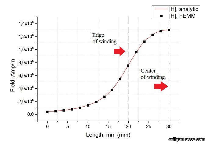
Fig. 3. Axial field intensity. Countdown from a point situated at 30 mm from the center of the coil which length is 20 mm. Thus, the edge of the coil is at 20 mm from zero, the center is at 30 mm.

What can we say looking at this graph?

First, the field strength in our devices is very high - in this particular case, it reaches 1.3 million Amperes/meter, which corresponds to the field induction in air of more than 1.6 Tesla. This is quite at the level of the most powerful laboratory installations (however, they are more often about constant fields, and in our case these are pulse values: maximum constant current for the selected wire is only 5 Amperes, at 100 A it will burn out in less than a second). Among other things, these results suggest that the use of an additional magnetic core in high-power coilguns is inappropriate, since ferromagnets almost lose their magnetic properties in such fields (I got the same conclusion here using numerical modeling of some cored systems).

Secondly, it can be seen that the field decreases rapidly when moving away from the coil - the voltage is already only about 10% of the maximum at a distance from the edge of the winding equal to its inner diameter, and at twice the distance it is almost zero. This fact demonstrates that the size of the area in which the force interaction of the coil and the ferromagnet occurs is very limited. We will talk about this in more detail in one of the following articles devoted the optimal proportions of accelerating windings in a coilgun.

Let us now return to an interesting question raised at the beginning of this publication, namely: what is the field of a cylindrical winding at an arbitrary point that does not lie on its axis? We, as gauss-builders, are primarily interested in the space enclosed within the cylindrical region formed by the inner surface of the coil - there is a barrel in which a ferromagnetic projectile moves which is accelerated  by the coilgun (see Fig. 4). It is intuitively clear that for the projectile inside the coil, the absolute value of the intensity vector will increase with the distance from the centerline, because we will be closer to one of the edges of the coil, which forms this field with its currents. On the other hand, when moving away from the axis of symmetry, the field should acquire a radial component, which is generally uninteresting and even harmful, because, instead of accelerating the projectile in the longitudinal (axial) direction, this vector will only destabilize its movement.

Fig. 4. Schematical drawing of the flus density vector inside a coilgun on its axis, and in a point situated closer to the inner surface of a coil. An axial (B_a) and radial (B_r) component of the latter vector are shown.

The exact solution for the shape of a field at an arbitrary point has a much more complex form than eq. (3) and given by so-called "elliptic" integrals - it is not expressed in terms of analytical functions and can be found in the special literature. For our illustrative purposes, I used FEMM modeling. In this case, the same system was considered as in Fig. 3 at the same current of 100 A (see Fig. 5). Here and further, for convenience, the flux density B will be depicted, instead of H (which is of orders of hundreds of thousands and millions of A/m).

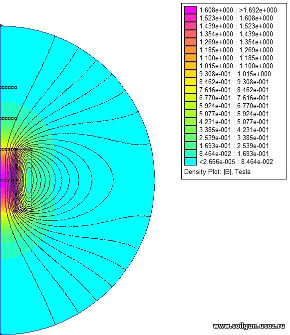
Fig. 5. Flux density graph produced by FEMM.

As usual for axial-symmetrical systems, FEMM models only one half-plane, i.e. half of the section of our model - the second one is obtained by reflecting the drawing relatively to the origin (the left vertical border of the model). The graph contains extra points that were added into the model to build a field profile along the axis of the solenoid (they form lines at a distance of 0, 1, 2, 3, 4 and 5 mm along the axis, i.e. the first line coincides with the axis of the coil, and the last line coincides with its inner surface), as well as radial field profiles (in the center of the winding, in the plane coinciding with the end of the coil at a distance of 10 mm from the center, then at a distance of 20 and 30 mm from the center). Below are the result (see Fig. 6, 7).

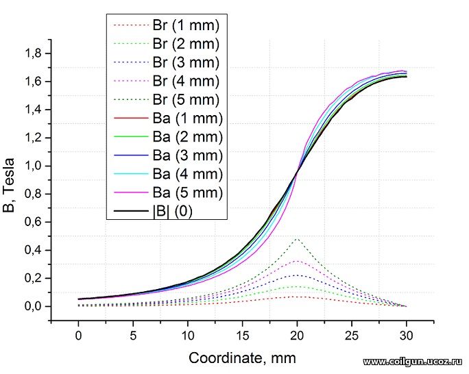
Fig. 6. Axial and radial components of the flux density vector along the lines situated at distance from 1 to 5 mm from the axis. Black is the density on the axis itself (the radial component is zero there, and a module of B equals to B_a). 

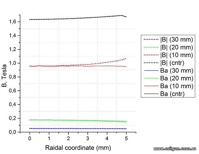
Fig. 7 Radial distributions of the module of the flux density vector (|B|) and its axial component (B_a) in planes corresponding to the center of the coil (cntr), its edge (10 mm), and also at 20 and 30 mm from the center.

What conclusions can be drawn from these illustrations? The most important one is this: the axial component of the magnetic field changes quite little with deviation from the center of the barrel (coil). Fig.6 shows that these variations do not exceed 10% of the induction value on the axis (|B| (0)). The greatest deviation, as expected, takes place near the inner wall of the coil (radial coordinate 5 mm) - there is the strongest radial component of the vector B, which takes the maximum value in the plane coinciding with the end of the winding (longitudinal coordinate 20 mm).

Hence, for various estimations (including for the forces acting on the projectile in accordance with the formulae of the previous publication), we may not calculate the field over the entire cross-section of the projectile, but with acceptable accuracy replace it with the field strength on the axis. The latter value can be simply determined by eq. (3) and (4).

We can also notice an interesting feature of the behavior of the magnetic flux density vector (or intensity, it does not matter in this case): when moving away from the axis of the solenoid, it decreases if we are talking about points lying outside the coil, but increases if we consider the area inside the winding. However, as already mentioned, these variations are insignificant.

In the next publication, we will consider such an interesting question as determining the shape of the coil for the most effective acceleration of the projectile.

Literature:

[1]. Карасик В. Р., «Физика и техника сильных магнитных полей», М., "Наука" 1964 г., 348 стр.