| Home » Articles » Theoretical papers » Coilgun calculations |
In this article, I promised that I would try to analyze in more detail the dependencies that are derived from the analytical relations for fields and forces acting on a ferromagnet in an electromagnetic accelerator. Let's start by rewriting these relations. It is established here that the force acting on a cylindrical projectile with a length l and a cross-sectional area S, drawn into magnetic field with a dependence on the coordinate H(x), can be expressed as follows:
F = Bнас ·S ·[H(x+ l) - H(x)] (1)
Another publication shows that the magnetic field on the axis of a multilayer solenoid of length 2b, consisting of N1 layers of N2 turns in each layer, and having an inner radius a1 and an outer radius a2, for a point with coordinate z from its center has the form:
In the same place, I demonstrated that the field changes very little when it deviates from the axis of the coil, and for calculations using the formula (1), the value of H determined in accordance with (2) can be used with good accuracy. These relations are sufficient to obtain very interesting conclusions about the properties of electromagnetic accelerators.
1. Pulling force for an infinitely thin and arbitrary shaped projectile. Let's start with trying to get a formula for the force pulling a body of any geometric shape (not only a cylindrical object, described by eq. (1)) into the coil. To do this, first consider such an abstraction as an" infinitely thin" projectile. Directing the length of the core to zero in (1), we get an element of force acting on such a" pancake-like " body in the following form:
where dH is the differential (increment) of the magnetic field when the coordinate is shifted by dx. This formula will be useful to us in the future - with the help of it we will get a very important estimate for the maximum achievable speed of the projectile in the coilgun.
The following is quite simple - any body can be represented as a set of infinitely thin sections, the shape (area) of which changes as it moves along the body (see Figure 1). It is more convenient to denote as x the coordinate of the point closest to the coil (i.e., the nose of the projectile). Then, replacing the coordinate designation with y in relation (2) and integrating along a body of length z having an arbitrary cross section S (y), we obtain the following formula:
With the help of this ratio, it is possible to estimate the attractive force for any bodies, and a particularly simple description is obtained for bodies of rotation (which, in fact, is most relevant for projectiles). For example, for a spherical core the following description of the force is obtained:
And for a cylindrical body with a base area of S:
that is, as expected, we again got the formula (1).
2. Determination of the velocity and kinetic energy acquired by the projectile when it is drawn into the coil. Let's rewrite the formula (2) in a more convenient form, changing the notation. The coordinate of the projectile x will be counted from the end of the coil (the closest to the attracted body), the inner and outer diameters of the coil will be denoted as d and D, respectively, its length will be c. We will also introduce a coefficient a, equal to the ratio of the wire's "copper gauge" b to its diameter in isolation (usually when winding, a ≈ 0.75...0.85). Then
Here, the field is measured in units of A / cm, values of D, d and c - in centimeters, and b - in millimeters. As mentioned earlier, such a record is not very convenient, because the current flowing through the coil i can take different values depending on the wire gauge and the applied voltage, so it is more logical to take the power P of the supply as a parameter. Then, the limiting current through the winding will be determined by the well-known expression
where R is the ohmic resistance of the wire, which, in turn, for a cylindrical winding with the parameters specified above, makes
where δ is the resistivity of the winding conductor (for copper, δ ≈ 0.0175 Ohm·mm2/m). In order to estimate the kinetic energy and the speed that the projectile obtains, it is necessary, generally speaking, to know the dependence of the current flowing in the coil on time, which is determined by many factors - the inductance of the winding, the properties of the power source (if we are talking about a capacitor - its capacity and internal resistance), the parameters of the commutator used for switching and the electrical circuit, which is used to damp the EMF of self-induction when the current is interrupted. In addition, the moving ferromagnetic projectile itself induces an inductive EMF in the coil, which can be added or subtracted from the supply voltage of the circuit. In order not to consider these factors, which are individual for each coilgun, we will make a number of simplifying assumptions. First, we neglect the influence of the core on the shape of the current. As practice shows, this is all the more true, the lower the velocity of the projectile and the greater the field strength (i.e., the energy "pumped" into the coil when fired). Secondly, we will assume that the current in the coil after switching on instantly reaches the maximum value determined by eq.(6), and immediately after switching off it drops to zero (i.e., the current pulse has a rectangular shape in time, see Fig. 2a). This situation is an abstraction, because in a real coil, the inductance does not allow the current to change instantly. As a result, the coil has to be "activated" with a certain margin in time before the moment when the projectile reaches an area where a noticeable retracting force acts. Because of this, some of the energy is spent almost uselessly - the current is already flowing through the coil and warming the wires, and the projectile is not really attracted yet. Disconnection also has to be performed in advance - the best moment for it would be the point (so - called "zero point", ZP) , when the geometric center of the projectile coincides with the middle of the winding - here the retracting force changes its sign and begins to suck the projectile back (see Fig. 2b). But due to the inertia of the processes, it is necessary to break the control switch with a certain margin, otherwise the current "tail" in Fig. 2a leads to slowing the projectile down (or, if we are talking about a system with an unbreakable switch, we should design it in such a way that the current in the ZP is already quite small).
Fig. 2. Idealized (—) and real (-------) current waveforms in a coilgun (a), and accelerating force profile acting on projectile (b).
In any case, it turns out that in a real system it is not possible to use the entire region of space (it is located in the left half-plane in Figure 2b), where the effective acceleration of the body occurs. In our approximation, this is possible, because we are able to instantly turn on and de-energize the coil at the optimal time. So, we will have the most favorable (optimistic) estimates for the energy and speed of the projectile, which, in fact, we need. We can end these arguments by saying that our abstract case approximately describes the situation in an RLC circuit with a supply capacitor of a very high voltage and capacitance - then the current rise front will be very steep, and the decline after saturation is reached will be very flat. Such a circuit must be commutated by a switch with an infinite permissible voltage - then it can instantly interrupt the current. That is, we are talking about a certain "ideal coilgun". As is known from the physics course, the increment of kinetic energy can be calculated through the profile of the force acting on the body F (x), integrating it along the acceleration trajectory between the starting and ending points x1 and x2:
If we assume that the accelerated body has a cylindrical shape with a base area of S ≈ πd2/4 (i.e., the barrel walls are very thin and the caliber of the projectile is equal to the inner diameter of the coil), then substituting the relations (4), (5) - (7) into (8) , we will get:
where the "geometrical" function is
the form factor of the coil (which is in the formula (5) in square brackets) is indicated by h
As can be seen, the maximum kinetic energy derived is proportional to the saturation induction of the accelerated ferromagnet, the winding density coefficient, as well as the square root of the ratio of electric power and resistivity of the wire that the coil is wound with (while it does not depend on the diameter of this wire). The f function contains all the geometric properties of the system, including the start and end points of acceleration x1 and x2. Everything is unambiguous with the end point - as shown above, it must coincide with the ZP, which, as it is easy to show for cylindrical coils of length c and a projectile of length z, is given by the expression x2 = - ½(c+z). As for the starting point, there may be different approaches. Obviously, in order to estimate the maximum energy Emax that the projectile can get, its acceleration should begin with an infinite distance from the coil (x1 = ∞). In this case, however, the acceleration will last indefinitely, and its efficiency will be zero (since the loss power is constant and equal to P). In real coilguns, the coil is usually activated at the moment when the projectile enters it with its nose, or somewhere near this point (x1 = 0). Let's take this case as closer to practice (E0), and consider it along with the previous one for illustration. Then, taking (9) into account:
Having determined the kinetic energy received by the projectile, it is possible to estimate its speed or, more precisely, its increment Δv on the coil under consideration. Let us assume two extreme cases with respect to the initial (before switching on the current) velocity of the projectile v0: acceleration of the projectile from a rest or very slow movement (v0 << Δv), and with a high initial velocity (v0>>Δv). We denote the corresponding increments of velocity as Δv0 and Δv∞. The first case, obviously, corresponds to the starting stage of the accelerator, the latter - to the coil located somewhere closer to the end of the barrel of a multi-stage coilgun. Recalling the well-known "school" formula for the kinetic energy E = ½mv2 and remembering that v=v0+Δv, we have for the energy obtained by the projectile from the considered stage: ΔE = ½m (v2-v02)= ½m (v-v0)(v+v0)=½mΔv(2v0+Δv), hence
The mass of the accelerated cylinder with length z and density p can be easily expressed in terms of its dimensions: m = z·ρ·πd2/4. Then it follows from the relation (9) that:
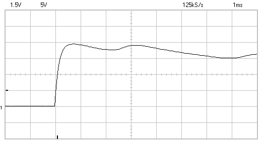
It follows from eq.(14) that the velocity increment given to the projectile during acceleration from a state of rest is proportional to the root of the fourth power of P, and at a high initial velocity - to the square root of P. Interestingly, on the page of relations for electromagnetic accelerators, I obtained from simpler considerations that, in general, for a coilgun operating in the DC mode and uniformly accelerated motion of the projectile, the output speed is proportional to the cubic root of P, which corresponds well to the "golden mean" between the two extreme cases discussed above. Using the relations (12), it is also possible to obtain expressions for the increment of the velocity of the projectile accelerated from an infinite distance from the coil (x1 = ∞, this will be the maximum speed achievable in a coilgun of this configuration), and from any specific point x1. The estimates made by formulas (12) and (13) should have a fairly good accuracy (as far as the relations (1) and (2) at the beginning of this article are valid). It would seem that knowing the expressions for the velocity and energy of the projectile, it is easy to estimate another key parameter of the coilgun - its efficiency. However, it turns out that this is not the case. The fact is that for this it is necessary to know the energy Eext = P·t0 spent from an external source during the time t0 of acceleration of the projectile, and this is difficult to do, and for various reasons in different cases. At zero initial velocity, we will not know t0 , since the law of motion of the projectile x (t) is determined not only by the constant value of the power acting in the circuit P, but also by the profile of the acting force (10). As a result, to estimate t0 in each case, it is necessary to perform a numerical modeling - it cannot be expressed in a simple analytical way. For a high initial velocity v0, it seems that it is possible to take the duration of movement through the coil (with length c) as a constant value t0 ≈ c/v0 and get the efficiency in the form of some value proportional to v0, as done here. As a result, we can draw an absurd conclusion that the efficiency of the coilgun will tend to infinity with an increase in the speed of the projectile.... The reason for this misconception is simple - when deriving the equations (1), (5) and (9), we neglected the influence of the projectile itself on the magnetic field of the coil and considered the power dissipated in the circuit constant, and this is true only at a low speed of the body and strong (and constant) currents in the winding. But with a high value of v0, the coil current (with a constant number of turns) will not have time to increase to values close to (6) due to the influence of inductance - that is why in multistage systems, as the number of stages increases, they are wound with an increasingly thicker wire, or they contain fewer turns. In addition, as we mentioned above, a rapidly moving projectile produces an inductive EMF in the coil, which can have a significant effect on the shape of the current in the circuit. At one time, I even used this effect to build an original induction sensor for the position of the projectile in the accelerator barrel. The figure below shows the current waveforms obtained when working with this sensor - they show the characteristic vibrations caused by the movement of the ferromagnet inside the coil.
Fig. 3. Current oscillations in a coil with fastly moving ferromagnet inside caused by inductive EMF.
Thus, with an increase in the initial velocity of the projectile, the "DC" and "strong field" approximations lose their validity, and to determine the efficiency, again, it is necessary to use numerical modeling.
| |||||||||||||||||||||||||||||||||||||||||
| Views: 525 | | | |||||||||||||||||||||||||||||||||||||||||


| Total comments: 0 | |