| Home » Articles » Theoretical papers » Coilgun calculations |
Introduction.
At the end of last year, I completed a rather serious mathematical study of accelerators of ferromagnetic bodies based on basic equations for fields and forces in electromagnets. As a result, these articles were published, and a new criterion was proposed for a comparative assessment of the quality of gauss guns - so-called G-factor. With its use, I compiled a special Table where I placed all the currently known designs of multi-stage coilguns, for which the necessary information was available (by the way, this table is open for updating with fresh data, so all gauss-builders are welcome ...). The analysis of the Table, which I did on New Year's holidays, revealed certain patterns, among which were the parameters of two types of coilguns outstanding in terms of speed and efficiency, namely, with a spherical projectile, and also one built on the principle of a "traveling wave" (TW). And if the high speed characteristics a ball, in principle, followed from my calculations and were not unexpected for me, I had to write a separate article to analyze the "wave" coilgun.
What is a TW coilgun?
To begin with, I want to remind you what is a "travelling wave" launcher. Imagine a conventional multistage accelerator (see Fig.1).
The traditional way of functioning of this system is as follows: each coil turns on at the moment when the accelerated body approaches its front face, and turns off when the projectile reaches some optimal point. Then the next winding is triggered and so on. It is not difficult to understand that in this case the accelerating force is extremely uneven, since the projectile periodically falls from the area of a strong field to a weak one and vice versa. Moreover, since the current in the inductors is not able to change instantly, a situation may arise when the previous coil is already starting to slow down the projectile, and the subsequent one cannot accelerate it properly yet, because the current in it has not had time to "build up" or the projectile has not yet entered the area of effective retraction - as a result, the total force becomes negative, i.e. the speed of the body decreases (see the upper graph in the animation Fig. 2). The picture can be improved by dramatically increasing the number of coils, and activating several of them at once so that the total field created by them forms the area of maximum acceleration for the projectile. As a result, the average accelerating force increases and becomes more stationary (Fig. 2, below). During its movement, the ferromagnetic body is accompanied by a kind of "wave" of the magnetic field, which moves with it (hence the name of the structure).
Fig. 2. The principle of operation of a conventional multistage accelerator (top), and a TW coilgun (bottom). The right part schematically shows the dependencies of the force acting on the projectile (F) vs time (t).
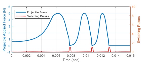
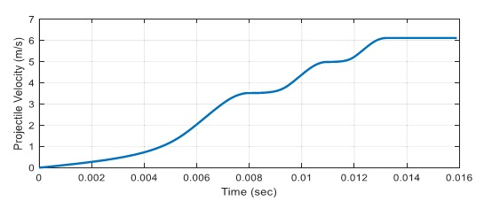
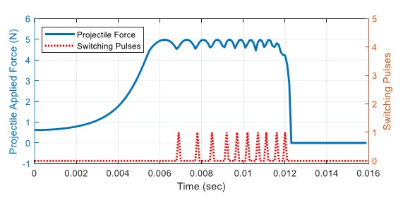
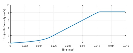
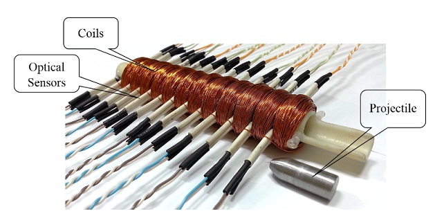
It is not surprising that this configuration is considered by many as a kind of "Holy Grail" of gauss- construction (and with good reason). However, its high structural complexity leads to the fact that there are only a few really tested models, the mere fact of assembling them inspires respect for their creators. One of such rare examples is Dantist's DB6L mentioned in the Introduction. It should be noted that this (rather obvious) approach is periodically "rediscovered" by various researchers and presented as a kind of innovation. For example, see [1], in which a small accelerator with a voltage of 24 V is investigated. As a result of increasing the number of windings from 3 to 12 (at a fixed acceleration length) and switching to a "traveling wave" scheme, the authors managed to increase the efficiency by almost half, and the speed by a third. Below are some illustrations from this article.
The calculation.
Now let's get down to the main task of our research - let's try to determine the maximum achievable projectile velocity and efficiency in the TW accelerator. To do this, we will use the relations obtained in the works devoted to the study of conventional single- and multi-stage accelerators (these functions are quite difficult to perceive "from scratch", so I would recommend you first to familiarize yourself with these publications). They can be used with one significant simplification - earlier we introduced everywhere two variables that described the coordinates of the accelerated body relative to the individual winding, at which the current is switched on and off, respectively. It is easy to realize that in the case of a TW accelerator, these variables disappear from consideration, since the constant switching on and off of many small windings forms one "virtual" coil, which is always in the same position relative to the projectile and moves along the barrel with it (see the animation in Fig. 2). Then, if we denote this position (coordinate) as x, then all integral expressions from the formulas disappear, and we get for the output velocity v of a projectile of length z and cross-section S, acquired in a coilgun of length l :
where the magnetic field is described by the following equation:
The meaning of the parameters included in the formula is: a - the dimensionless ratio of the caliber of the winding wire "by copper" b to its effective diameter in insulation (usually a = 0.75..0.85 is obtained) Bнас - saturation induction of the projectile material, Tl i - current, Amps D - is the outer "virtual" coil dia, cm d - coilgun caliber - inner diameter of coils, cm c - the length of the "virtual" coil, cm. It is more convenient to translate all the geometric parameters of the system into a dimensionless form, expressing them through the accelerator gauge d: D = α·d, c = β·d, z = γ·d, x = φ·d (see fig. 1 and 4).
Fig. 4. The scheme of designations of geometrical parameters for the conventional accelerator. In the case of TW, the current strength and the position of the projectile are constant, so the relative coordinate φ will be the only one.
Thus, oddly enough, calculations for a structurally extremely complex TW coilun are much simpler than for traditional devices. Modifying the relation (1) as it is done here, we obtain finally for the maximum achievable output speed:
and for the efficiency:
where the geometrical multiplier depends only on one coordinate now :
and Y function, is as earlier a dimensionless expresson of the form-factor of the ("virtual") coil:
The other parameters remain: δ - is the resistivity of the winding conductor, Ohms *mm2/m E - is the electrical energy expended on the shot, J ρ - the density of the projectile material, kg/m3 As can be seen, relations (3) differ from similar formulas for conventional multistage accelerators only in the form of a geometric multiplier Uf (see figures (9) and (11) of this article, they featured a multiplier Wf). Therefore, to find the maximal v and η, it is necessary to go the same way - try to maximize Uf and Uf 4/3 ·γ, respectively. If this is done, it turns out that the limit value of Uf is 0.329 and is achieved with the following set of parameters: γ = 0, α = 1.77, β = 0.817, φ = - 0.883. That is, the optimal projectile here will be infinitely thin, too. The table below shows comparative numerical values for the system with the previously considered parameters, namely: energy E = 500 J, coils of caliber d = 0.8 cm wound with copper wire with an average density a = 0.8, iron projectile (Bнас = 2 Tl, p = 7870 kg/m3).
The coincidence for the two systems looks inexplicable. Perhaps these two varieties, into which I arbitrary divided the accelerators, are not so far from each other in principle - after all, in real designs, activation of neighboring coils may well be carried out with some "overlap" (that is, there is a range of projectile coordinates where they work simultaneously). Or, the idealization of the current shape in coils in the form of rectangular pulses used in my models affects here - taking into account the rise and fall times would probably lead to a change in the whole picture... In any case, there is still something to think about....
As for the patterns describing the impact on the speed and efficiency of the main parameters of the coilgun, they remain in force and are described in the finale of this article.
Sincerely Yours,
[1]. A.Hassannia and K.Abedi, "Optimal switching scheme for multistage reluctance coilgun", IEEE Transactions on Plasma Science, vol. 49, 3, 2021.
| ||||||||||||||||||||||||||||||||
| Views: 252 | | | ||||||||||||||||||||||||||||||||
| Total comments: 0 | |